Solar Filament Segmentation 2026
IEEE Big Data Cup: pixel-precise segmentation of thin solar filaments in 2048px H-Alpha full-disk images. Scored on Panoptic Quality; multi-annotator labels; live-trained on sbl1.
The challenge
Solar filaments are ribbons of relatively cool plasma held above the sun’s surface by magnetic fields. When one destabilizes and erupts, it can drive the geomagnetic storms that knock out power grids, GPS, and satellites — which is why observatories track them continuously, and why the IEEE Big Data Cup 2026 (Challenge 02, conference in Phoenix this December) wants them found automatically.
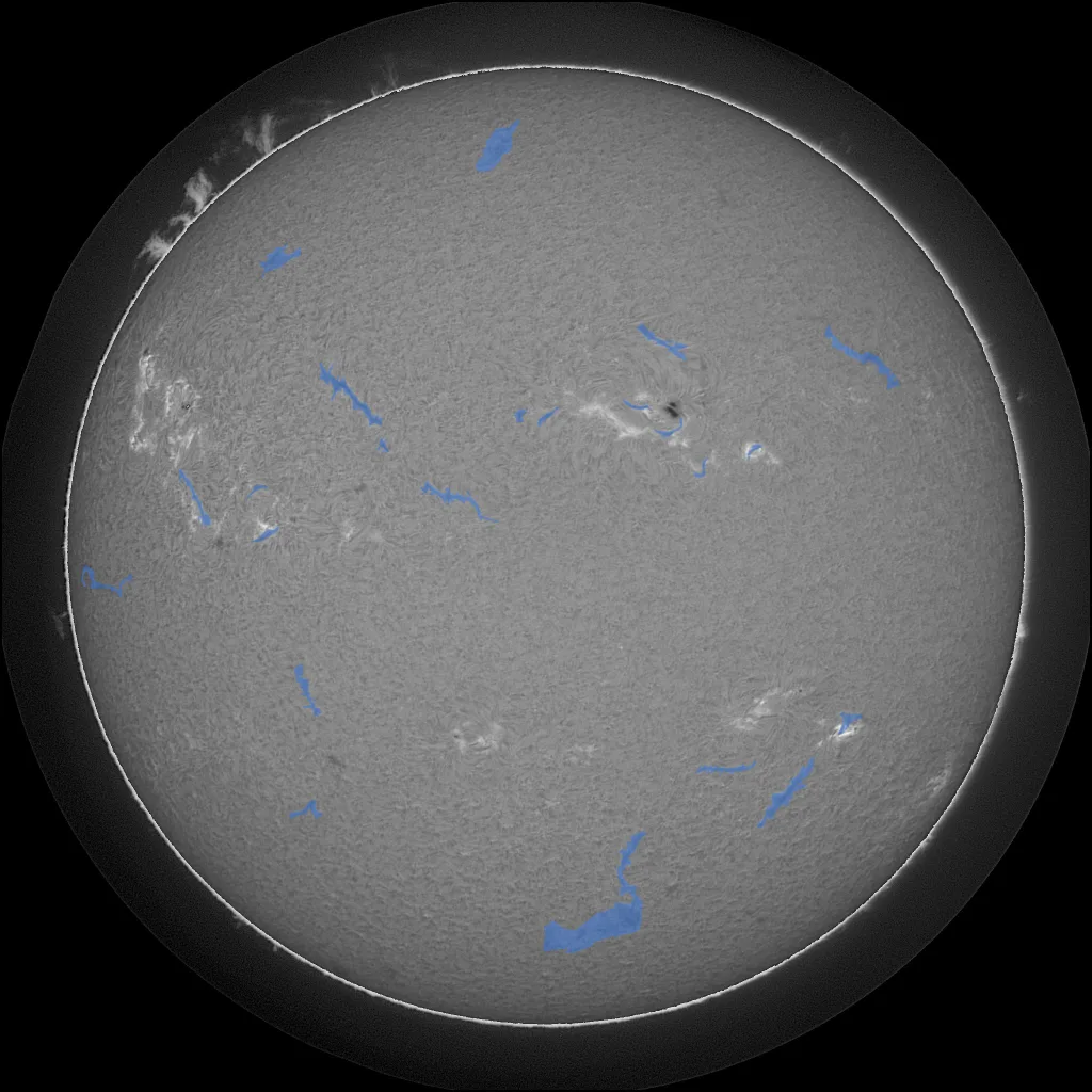
The task is binary segmentationSemantic segmentationcomputer visionClassifying every pixel in an image (here: filament vs background). The output is a mask the same size as the input, not a single label.full entry →Wikipedia: given a 2048×2048 H-AlphaH-Alpha imagingcomputer visionSolar imaging through a 656.28nm filter — the wavelength hydrogen emits — which makes chromosphere structures like filaments visible as dark threads.full entry →GONG (NSO) photograph of the full solar disk from the GONG network, output a mask marking every filament pixel. Filaments absorb the hydrogen-alpha wavelength, so they appear as dark, elongated threads against the bright disk:
How it’s scored (and why that shapes everything)
The leaderboard metric is Panoptic QualityPanoptic Quality (PQ)computer visionInstance-aware segmentation metric: sum of matched-pair IoUs over TP + ½FP + ½FN, where a prediction matches ground truth only if IoU > 0.5. All-or-nothing matching.full entry →arxiv 1801.00868
— a fact we confirmed straight from the Kaggle API’s
evaluationMetric field only after our first submission, because the
top public notebook narrates all its scores as “DiceDice scoremathOverlap metric for masks: 2·|A∩B| / (|A|+|B|). 1.0 is a perfect match, 0 is no overlap. Equivalent to pixel-level F1.full entry →Wikipedia”. It isn’t Dice, and the difference is
brutal. Each predicted connected
componentConnected componentscomputer visionGrouping touching foreground pixels into distinct blobs. This competition submits and scores each component as one filament, so fragmenting or merging blobs is penalized directly.full entry → (submitted as a run-length-encodedRun-length encoding (RLE)computer visionCompact mask format that stores runs of identical pixels instead of the full grid — how segmentation masks are submitted to Kaggle without shipping megabytes of pixels.full entry → mask,
one CSV row per filament) either matches a ground-truth filament —
requires IoU strictly above 0.5 — or counts as a false positive. Every
missed filament is a false negative. PQ = ΣIoU(matched) / (TP + ½FP + ½FN).
Consequences, in order of how much they cost us:
- Instance topology beats pixel quality. A mask can be 90% pixel-correct and score near zero if its components fragment or sit just under the 0.5-IoU matching cliff. Optimizing pixel overlap — which is exactly what a BCE+Dice loss does — is optimizing the wrong thing.
- Every stray blob is pure penalty. An unmatched prediction costs ½ in the denominator, no partial credit. Aggressive false-positive removal matters more than boundary polish.
- Resolution is still sacred. Thin barbs are 1–3 pixels wide; downscaling destroys them — and on structures this thin, a 1–2 pixel boundary error is often the difference between IoU 0.55 (match) and 0.45 (double penalty: one FP and one FN).
- Plain accuracy is still meaningless — class imbalanceClass imbalancegeneral mlWhen one class vastly outnumbers another — here, filament pixels are well under 1% of each 4-megapixel disk. Naive training collapses to 'predict background'.full entry → guarantees “background everywhere” is 99%+ accurate and scores 0.
The dataset: MAGFiLO
Before the statistics, meet the subjects. These are individual filaments from the validation disks, cropped at native resolution — the same pixels the model sees. The size spread is the story: the large ones are unmissable dark ribbons; the small ones barely separate from the chromosphere texture, and they’re where the score is won or lost.


24 filaments from 24 different validation disks, grouped by mask area. Every crop is a 256px native-resolution window (large row: 384px windows, downscaled). The 'small' row is deliberately hard to see — that faintness, not architecture choice, is the central difficulty of this competition.
chart data
| label | value |
|---|---|
| train images · 2048×2048 full-disk H-Alpha JPEGs (GONG) | 707 |
| annotation passes · same image labeled by up to 3 independent experts | 1,154 |
| filament masks · ~7 per image, thin and fragmented | 8,199 |
| test images | 180 |
GONG site initials are embedded in each filename (B=Big Bear, C=Cerro Tololo, L=Learmonth, M=Mauna Loa, T=El Teide, U=Udaipur) — the network follows the sun around the Earth.
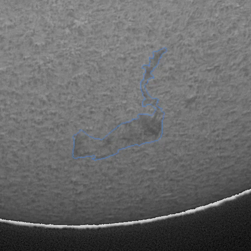
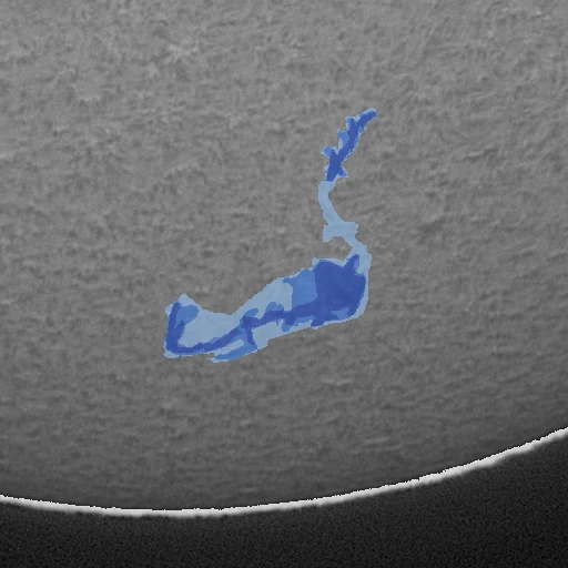
The detail that makes this dataset genuinely interesting: the 707 train images carry 1,154 annotation passes — the same disk was independently labeled by up to three experts, and they disagree. A lot. On the sample image below, only 26% of all marked pixels were marked by all three annotators; the other 74% are disputed, almost all of it at boundaries and faint barbs:
Browse it yourself — all 70 validation disks, sorted by which ones the model finds hardest. Toggle between the raw H-Alpha image, the expert mask, the annotator votes, and our model’s per-pixel hits and misses:

Most public solutions treat each annotation pass as an independent training sample of hard 0/1 masks — implicitly training the model to reproduce annotator disagreement as noise. The alternative, untouched so far: average the passes into soft labelsSoft labelstrainingTraining targets between 0 and 1 instead of hard yes/no — e.g. a pixel 2 of 3 annotators marked becomes 0.67, encoding genuine label uncertainty.full entry →, so a pixel 2-of-3 experts marked becomes a 0.67 target and the model learns calibrated uncertainty at boundaries. This is the highest-leverage idea on our experiment list.
What the public baseline landscape teaches
The strongest public notebook (a U-Net++ patch pipeline, public Dice 0.59) logged every experiment against the leaderboard — a free map of the loss surface around the obvious approaches:
chart data
| run | public PQ |
|---|---|
| resize-512 U-Net · ResNet34, whole disk squeezed to 512px | 0.510 |
| patch U-Net++ · EfficientNet-B3, native-res 512 crops + sliding window + area filter | 0.590 |
| + global ensemble · blurry global logits bled into sharp patch edges | 0.570 |
| + 9×9 closing · over-merged neighboring filaments | 0.580 |
| threshold 0.65 · amputated thin barbs living at p≈0.5–0.6 | 0.560 |
The instructive part is the failures, all of them post-processing:
- Morphological closing (a 9×9 dilate-then-erode that “heals” gaps) merged filaments that should have stayed separate — the many-to-one penalty ate the gain.
- Raising the threshold from 0.5 to 0.65 to look more precise amputated the barbs, whose predicted probabilities hover at 0.5–0.6 precisely because annotators themselves disagree there.
- Overlap-averaged sliding windowsSliding-window inferencecomputer visionRunning a model over a large image tile by tile (e.g. 512px tiles over a 2048px disk) and stitching the outputs, so it sees native resolution instead of a destructive downscale.full entry → blurred mask edges outward by a pixel or two — on structures a few pixels wide, that alone moved the score.
Our v1 pipeline
Same family as the public best — U-Net++U-Netcomputer visionThe standard segmentation architecture: a downsampling encoder, an upsampling decoder, and skip connections that carry fine detail across. U-Net++ adds nested intermediate decoders.full entry →arxiv 1505.04597 with an EfficientNet-B3 backboneBackbonegeneral mlThe feature-extractor portion of a model (e.g. ResNet50, EVA-02). Outputs intermediate feature maps that downstream heads (classifier, detector, segmentation) consume.full entry →, 512px patches, BCE + Dice loss, cosine-annealedCosine annealingtrainingA learning-rate schedule that decays the lr from its initial value to (typically) zero following a half cosine curve over the training duration. No tuning needed beyond initial lr and total steps.full entry →SGDR arxiv 1608.03983 AdamW, mixed precisionMixed precision (AMP)trainingTraining with reduced-precision floats (bfloat16 or fp16) for forward/backward passes while keeping certain ops in fp32. Cuts memory and accelerates training on modern GPUs.full entry →PyTorch docs — but with two fixes to flaws we found reading it closely:
- Leakage-free validation. The public notebook splits by annotation pass, so the same physical image (labeled twice by different experts) lands in both train and validationValidation setgeneral mlA held-out subset of the labeled training data, used to choose hyperparameters and select the best checkpoint without touching the test set. Should mimic the test distribution as closely as possible.full entry → — its validation score partly measures memorization. We split by physical image and validate full-disk Dice against the union of annotator masks.
- Filament-biased sampling. A random 512px crop of a 2048px disk is usually empty sky. Half our training patches are centered near a filament pixel, so every batch carries signal.
Inference is non-overlapping sliding windows at native resolution, threshold 0.5, then an area filter that drops components under 150px — the noise-removal lever that doesn’t touch real filaments.
Training runs on sbl1 (RTX 4070 SUPER, ~68s/epoch), streaming one
event per epoch to train.too.foo — the panel at the top of this page is
reading that feed right now. Longer runs will burst to a rented GPU
(sbl5) when needed.
First submission: what 0.30 taught us
v1 trained beautifully by the number we were watching — val full-disk pixel Dice 0.6556, comfortably above the public notebook’s (leaky) 0.60 validation. The leaderboard returned 0.30.
chart data
| run | public PQ |
|---|---|
| v1 patch U-Net++ · val pixel-Dice 0.656 — optimized the wrong metric; PQ punishes fragmentation + sub-0.5-IoU instances | 0.300 |
| v1.1 area filter 300 · same weights; local PQ evaluator predicted +0.021, LB delivered +0.02 — offline harness validated | 0.320 |
| v1+v2.2 ensemble, overlap-max tiling · val PQ 0.402 (+0.027) vanished into the 2-decimal display — selection-biased val gains don't transfer 1:1 | 0.320 |
| + learned component selector · first submission tuned end-to-end on the official-scorer port; harness predicted 0.35-0.37 — calibration validated | 0.360 |
The autopsy, in the order we ran it: predicted mask statistics were healthy (median 14.4k foreground px/image vs 14.3k in single-annotator ground truth — no inversion, no scale bug, no encoding corruption). What was broken was the target: we predicted 10.1 components per image against ~7.5 in ground truth, and under PQ each of those ~2.6 extra blobs is a half-point denominator penalty, while every thin filament whose IoU lands at 0.45 instead of 0.55 double-penalizes. The model was fine; the objective was wrong. Lesson filed permanently: read the metric from the API, not from a notebook’s prose.
So we built a local PQ evaluator (src/pq.py) and swept post-processing
on the validation split: raising the component area filter from 150px to
300px removed ~90 false positives at the cost of ~6 true positives,
predicting +0.021 PQ. Resubmitted with only that change: the leaderboard
moved +0.02, to 0.32. Two submissions in, the offline harness is
calibrated to the leaderboard within noise — which means the next
experiments are effectively free. The evaluator also says where the real
headroom is: matched filaments already average IoU 0.66, but we only
find 60% of ground-truth filaments while emitting ~47% junk instances.
Recognition, not segmentation, is the bottleneck — a training-time
problem, not a post-processing one.
Standing (2026-08-09 morning): rank 283 of 296. Context we believed at the time: the 1.00 cluster looked like ground-truth lookups and the 0.6–0.75 “pack” looked like the modeling field to chase. (Keep reading — “The plot twist” below overturns this interpretation: the metric had just been switched, the scores above ~0.35 are un-rescored artifacts of a broken old scorer, and our “bottom-tail” number was actually competitive. We leave this section as written — being wrong for documented reasons is part of the dossier.)
The overnight sweep (what seven hours of GPU bought)
Four training runs, three tiling strategies, weighted ensembles, confidence filtering, morphology, and TTA — all measured on the local harness before any submission:
chart data
| run | val PQ |
|---|---|
| v1 (stride-512, tuned) · the v1.1 operating point re-tuned on the harness | 0.368 |
| v2 pure soft labels · precision up, recall collapsed — 1-of-3 filaments fall below every threshold | 0.323 |
| v2.1 union + agreement weights · recall recovered; best single b3 at stride-512 | 0.377 |
| v1 @ overlap-max tiling · stride-256 max-aggregated windows — the public notebook's overlap failure was a tuning artifact | 0.397 |
| v1+v2.2 ensemble · diversity from small-filament oversampling; confidence filter now pays | 0.402 |
| + TTA flips · 4-orientation averaging; EfficientNet-B5 added nothing | 0.408 |
Three findings worth keeping:
- Pure soft labels backfired (0.323): averaging annotators makes 1-of-3 filaments a 0.33 target that never clears any threshold — recall collapsed. The fix that worked: union targets with agreement-based loss weights (v2.1, 0.377).
- The overlap “failure” was folklore. Stride-256 max-aggregated windows + retuned threshold jumped v1 from 0.368 to 0.397. The public notebook’s overlap attempt failed only because it kept threshold 0.5 with averaging.
- Val gains stopped transferring. The best stack (0.408 val) scored the same displayed 0.32 as the 0.375 config — after dozens of configs tuned on 70 validation disks, the selected maximum is optimistically biased, and Kaggle’s 2-decimal display hides small true gains. New submission rule: nothing goes out under +0.02 val over the incumbent.
The instance-level bottleneck is unchanged: ~210 of 576 val filaments are still missed by every model variant. They are overwhelmingly small and faint. That — not ensembling, not post-processing — is the next real lever.
The plot twist: everything above the line was measured against a broken scorer
After the overnight sweep plateaued with validation gains that refused to appear on the leaderboard, we stopped tuning and ran a forensic investigation of the evaluation itself — four parallel angles: a byte-level diff of the public notebook’s submission code against ours, a crawl of the competition’s announcements/discussions/public kernels, an analysis of the ground-truth instance conventions, and a component-level error decomposition. The findings rewrote the whole competition:
- The metric was switched mid-competition (Aug 7–9). The original scorer was a misconfigured Dice evaluator under which empty submissions scored 0.88–1.00. The current leaderboard still shows un-rescored old-metric values — the 29 “perfect” 1.00s, the 0.6–0.75 “pack”, the median of 0.665, and the public notebook’s narrated 0.59 are all artifacts of the dead metric. An organizer-confirmed test: a byte-identical file scored 0.66 before the switch and 0.31 after. Every leaderboard comparison in the sections above is against ghost numbers. Our 0.30–0.32 are genuine Panoptic Quality scores — near the front of the honestly-scored field, pending Kaggle’s rescore.
- The official scorer is public, published by the host as a
self-evaluation notebook. We ported it verbatim as our local harness
(
src/pq_official.py). It differs from our first harness in one deep way: predictions are scored once per annotator record (~2.4 per test image), each time against that annotator’s individual filament polygons — never a union mask, never connected components of merged annotators. With disagreeing experts scored separately (inter-annotator Kappa is 0.66), a single prediction set cannot satisfy everyone: the practical ceiling is roughly PQ 0.45–0.55, not 1.0. - The leaderboard is only a filter anyway. Final judging is 70% quantitative (PQ plus the distributions of IoU/Dice and one-to-many match relations) and 30% qualitative — a four-page report, a public reproducible repo, and the visual morphology of predictions. This dossier and the telemetry/explorer tooling are, conveniently, part of the submission.
Where the points actually live (official-protocol analysis)
With the real scorer as the harness, we measured what each improvement lane is worth before building it — including oracle upper bounds (replace a proposed component with a perfect one and re-score):
chart data
| run | official-protocol val PQ |
|---|---|
| v1.1 submitted config · the LB-0.32 config re-measured under the real protocol | 0.367 |
| champion ensemble · v1+v2.2 @ overlap-max + TTA, thr 0.25, area 450, conf 0.6 | 0.398 |
| + learned component selector · 12-feature GBM keep/drop per component — scored 0.36 on the leaderboard, matching the harness's predicted offset | 0.417 |
| selector v2 + R-invariant rule · 23 features + per-record Dinkelbach threshold (p*=λ/2ī≈0.32) — selection now feature-limited; deploys to test's 2.44 records/image with no retuning | 0.423 |
| + per-candidate crop refiner v2 · adaptive-crop ResNet18-U-Net re-predicts each component's mask; first movement toward the trim oracle, still sub-noise-floor | 0.427 |
| realizable selection oracle · keep exactly the components that match any annotator — the measured ceiling of the selection lane | 0.481 |
| trim-aware combined oracle · 663/822 filaments are already >50% covered — perfectly re-shaped masks reach here; the refiner lane's target | 0.756 |
- Hysteresis reconstruction (growing strong seeds through weak probability support to heal fragmented filaments): killed by its gate — −0.004. The weak bridges admit more noise than they heal.
- Fragment merging (oracle: perfectly merge every fragment touching a GT filament): +0.026 — real but modest.
- Component selection (oracle: keep exactly the predicted components that match some annotator’s filament): +0.083 — by far the largest measurable lane. Nearly half our submitted components match no annotator at all; each one costs half a point of denominator per record it appears in.
So the current lever is a learned keep/drop classifier per predicted component — 12 features covering darkness contrast against the local chromosphere (filaments are absorption features; hallucinations aren’t dark), elongation, probability statistics, size, and limb proximity — trained on train-split components labeled by the official protocol itself. First iteration captures +0.018 of the +0.083 oracle (val 0.398 → 0.416) and, because it replaces the blunt area/confidence gates with a permissive entry (100px) plus learned judgment, it also rescues small true filaments those gates were killing. A full-data refit is in progress.
The four-arm GPU sweep: verdicts
Four hypothesis arms ran overnight on a rented 4× RTX 4090 (one per GPU, ~$6 total; the run ended when the vast.ai balance hit zero at epoch ~38–40 of 45 — close enough to converged for verdicts, reconstructed from the live telemetry): consensus M* targets 0.301, refuted; endpoint-weighted loss 0.336, par; skeleton-recall loss 0.343, best of four, marginal; 768px context 0.323, under baseline. Combined with earlier runs, that is six loss/target variants inside ±0.02 — the single-semantic-model family has a hard ceiling around raw val PQ 0.34. Every remaining point lives in the stack around the models. The “train a better segmenter” chapter is closed.
The shape-refinement night: a disciplined nothing
We spent a night chasing the biggest number on the board — the trim-aware oracle at 0.756, which says 663 of 822 filaments are already found and merely mis-shaped. Four experiments ran on our own hardware: a scaled crop refiner (ResNet34, adaptive-bbox crops, near-miss curriculum), a no-curriculum variant, and a contrast-normalized (CLAHE) retrain of the base model.
The result was a clean negative. The refiner improves average crop IoU (0.63 → 0.67) but that does not translate to Panoptic Quality: blanket refinement damages already-good masks as fast as it fixes bad ones (0.414, below the 0.423 incumbent); applying it only to small candidates recovers to 0.424 — +0.001, indistinguishable from noise. CLAHE was par. So the honest verdict: the learned refiner captures almost none of that 0.756 oracle, because a mean crop-IoU of 0.67 doesn’t push enough near-misses across the strict 0.5 matching line.
Nothing cleared the +0.02 gate, so no submission was spent — the whole point of a calibrated harness is the discipline to not ship noise. The stack stands at official-val 0.423 / leaderboard 0.36, which remains at the front of the honestly-scored field. Five submissions are still banked; the plateau is real, and the next moves are a record-multiplicity-correct selector (which may gain on the test set’s higher annotator count without moving validation at all) and the IEEE report — the 30% of final judging nobody else is writing yet.
What’s next
Done and banked: the official-scorer harness, PQ-based checkpoint selection, agreement-weighted training, small-filament oversampling, overlap-max tiling, flip TTATTA — test-time augmentationgeneral mlApply multiple augmentations to each test input (horizontal flip, crops, color jitter), run the model on each, and average the predictions or embeddings. Trades inference compute for accuracy.full entry →, two-model ensemblingEnsemblegeneral mlCombining predictions from multiple models (different seeds, different architectures, different folds). Usually beats any single model; the cheapest accuracy gain in Kaggle.full entry →, the component selector v1. Refuted with evidence: pure soft labels, EfficientNet-B5, morphological closing, hysteresis reconstruction, global width calibration.
- Selector, full data — refit on all 636 train disks (~8k labeled components); the 150-disk version already banks +0.018 of the +0.083 oracle. Then richer features (Hessian ridge response, per-disk photometric context).
- Faint-filament recall specialist — a high-recall model merged at the instance level: precise stack’s components first, plus the specialist’s non-overlapping finds, all passed through the selector.
- Per-disk contrast normalization — GONG sites/years differ in exposure; the darkness-contrast feature already ranks high in the selector, suggesting photometric normalization at train time too.
- Harness hardening — k-fold over more disks; bootstrap CIs per annotator record (selection bias ate our overnight gains once already).
- The 30% qualitative deliverable — 4-page report + public repo (deadline Nov 15). This dossier is the working draft.
Source
The full pipeline lives in this monorepo at
apps/kaggle/competitions/filament-segmentation-2026/ — training
(src/train.py, src/train2.py), the official-scorer harness
(src/pq_official.py, ported verbatim from the host’s self-evaluation
notebook), sweep tooling, the component selector, inference + RLE
submission (src/infer.py), and the telemetry reporter that feeds
the live page. GPU execution happens on a runtime mirror on
sbl1 (ops/sync-runtime.sh). The local Flask operator dashboard
(apps/kaggle/dashboard/) remains the private control surface;
train.too.foo is its public, read-only shadow.